Did you hear about Machine Learning? Classification? Regression?

What's the difference between these tasks?

It all comes down to the data and the type of problem you want to solve. All Machine Learning algorithms use data.

Computers process numbers all the time, so any information you have needs to be represented as numbers. In the most basic form, each record is shown as an (x,y) pair in a 2 dimensional plane.

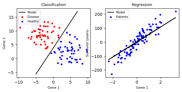
Classification vs regression

Then the task of classification is, given a new data point, does it belong to class blue or class red? Its output is a discrete value.

For regression, it tries to predict a continuous value. That's why there is only one color.

Is this hard to implement? Not really. The module sklearn comes with the algorithms out of the box. For classification or regression there are many examples available.

The program below creates the plots

#!/usr/bin/python3 
import matplotlib.pyplot as plt
import numpy as np

from sklearn.datasets import make_blobs, make_regression
from sklearn.svm import LinearSVC, LinearSVR


title_size = 14
axis_label_size = 12

params = {'legend.fontsize': 7,
          'figure.figsize': (7, 3),
          'axes.labelsize': 8,
          'axes.titlesize': 9,
          'xtick.labelsize': 10,
          'ytick.labelsize': 10}
plt.rcParams.update(params)


def make_classification_example(axis, random_state):
    X, y = make_blobs(n_samples=100, n_features=2, centers=2, cluster_std=2.7, random_state=random_state)

    axis.scatter(X[y == 0, 0], X[y == 0, 1], color="red", s=10, label="Disease")
    axis.scatter(X[y == 1, 0], X[y == 1, 1], color="blue", s=10, label="Healthy")

    clf = LinearSVC().fit(X, y)

    # get the separating hyperplane
    w = clf.coef_[0]
    a = -w[0] / w[1]
    xx = np.linspace(-5, 7)
    yy = a * xx - (clf.intercept_[0]) / w[1]

    # plot the line, the points, and the nearest vectors to the plane
    axis.plot(xx, yy, 'k-', color="black", label="Model")

    ax1.tick_params(labelbottom='off', labelleft='off')
    ax1.set_xlabel("Gene 1")
    ax1.set_ylabel("Gene 2")
    ax1.legend()


def make_regression_example(axis, random_state):
    X, y = make_regression(n_samples=100, n_features=1, noise=30.0, random_state=random_state)

    axis.scatter(X[:, 0], y, color="blue", s=10, label="Patients")

    clf = LinearSVR().fit(X, y)
    axis.plot(X[:, 0], clf.predict(X), color="black", label="Model")

    ax2.tick_params(labelbottom='off', labelleft='off')
    ax2.set_xlabel("Gene 1")
    ax2.set_ylabel("Survived (years)")
    ax2.legend()



random_state = np.random.RandomState(42)

f, (ax1, ax2) = plt.subplots(ncols=2)

ax1.set_title("Classification")
make_classification_example(ax1, random_state)

ax2.set_title("Regression")
make_regression_example(ax2, random_state)

plt.savefig("classification.vs.regression.png", bbox_inches="tight")

Machine Learning resources:

Machine Learning Classification vs Regression

Classification vs regression