YugabyteDB is a distributed SQL database that primarily focuses on high performance OLTP. The tables, and indexes, are split into tablets (with hash or range distribution on the key) with the goal to distribute them across nodes, to load-balance the reads and writes, with multiple replicas for high availability. This must involve cross-node operations because, to be consistent, each row has only on place where it can be concurrently read and written: the leader tablet.

An OLTP application has also many tables that are read frequently but rarely written. Those are often referred to as lookup tables, or reference tables. It can be the tables of countries, cities, currencies, article prices, and so on, small or medium size. For them you can accept that the writes take longer, being broadcasted to all nodes, in order to accelerate the reads, from a local table. You still want full ACID properties because you don't know when they will be updated, and don't want additional code, or change data capture, for this simple optimization.

There are some solutions for this in monolithic and sharded databases. Materialized view on Oracle can log the changes and propagates them, but on-commit refresh is not possible across databases. CitusDB has a table declaration for Reference Tables, which are table copies, on which all writes are propagated to all nodes with two-phase commit. Those work well in a distributed datawarehouse when those dimension tables are refreshed offline. But we need more agility for OLTP.

YugabyteDB, thanks to the two-layer architecture, implements this with multiple existing PostgreSQL and DocDB mechanisms:

redundant storage of table data, physically organized differently for performance reasons, and updated synchronously is, in a SQL database, done with an index on the table
PostgreSQL allows multiple indexes on the same columns
PostgreSQL supports covering indexes to allow Index Only Scan
PostgreSQL defines tablespaces to map physical attributes, like physical location, to tables and indexes
YugabyteDB can add placement info to tables and indexes
YugabyteDB doesn't need to read the table for Index Only Scan
YugabyteDB extended the cost based query planner to be cluster-aware

We call this technique "duplicate index" because the goal is to create multiple identical indexes and place them into each network location. It doesn't have to be replicated into each node. You may decide to have only one per Availability Zone for example, as cross-AZ latency is usually low.

My lab in docker-compose

For testing in a lab, that you can fully reproduce, I'm generating a docker-compose.yaml to simulate a multi-cloud, multi-region, multi-AZ cluster:

####################################################################
# creates a docker-compose.yaml to build a RF=$replication_factor
# cluster with $number_of_tservers nodes in total,
# distributed to the clouds / regions / zones defined by the list
# (to simulate multi-cloud, multi-region, multi-AZ cluster)
####################################################################

replication_factor=3
list_of_clouds="cloud1 cloud2"
list_of_regions="region1 region2"
list_of_zones="zone1 zone2"
number_of_tservers=8
number_of_masters=$replication_factor


{

cat <<'CAT'

version: '2'

services:

CAT

# counts the number of master and tserver generated
master=0
tserver=0
master_depends=""
# the masters must know the host:port of their peers
master_addresses=$(for i in $(seq 0 $(( $number_of_masters - 1)) ) ; do echo "yb-master-$i:7100" ; done | paste -sd,)

for node in $(seq 1 $number_of_tservers)
do
for zone in $list_of_zones
do
for region in $list_of_regions
do
for cloud in $list_of_clouds
do

# generate master service
[ $master -le $(( $number_of_masters - 1 )) ] && {

cat <<CAT

  yb-master-$master:
      image: yugabytedb/yugabyte:latest
      container_name: yb-master-$master
      hostname: yb-master-$master
      command: [ "/home/yugabyte/bin/yb-master",
                "--fs_data_dirs=/home/yugabyte/data",
                "--placement_cloud=$cloud",
                "--placement_region=$region",
                "--placement_zone=$zone",
                "--master_addresses=$master_addresses",
                "--replication_factor=$replication_factor"]
      ports:
      - "$((7000 + $master)):7000"
$master_depends
CAT

# the currently created is a dependency for the next one
master_depends="\
      depends_on:
      - yb-master-$master
"

}

# generate tserver service
[ $tserver -le $(( $number_of_tservers - 1 )) ] && {


master=$(($master+1))

cat <<CAT

  yb-tserver-$tserver:
      image: yugabytedb/yugabyte:latest
      container_name: yb-tserver-$tserver
      hostname: yb-tserver-$tserver
      command: [ "/home/yugabyte/bin/yb-tserver",
                "--placement_cloud=$cloud",
                "--placement_region=$region",
                "--placement_zone=$zone",
                "--enable_ysql=true",
                "--fs_data_dirs=/home/yugabyte/data",
                "--tserver_master_addrs=$master_addresses",
                "--replication_factor=$replication_factor"]
      ports:
      - "$(( 9000 + $tserver)):9000"
      - "$(( 5433 + $tserver)):5433"
      depends_on:
      - yb-master-$(( $number_of_tservers - 1 ))

CAT

}
tserver=$(($tserver+1))

done
done
done
done

} | tee docker-compose.yaml

I start this, connect to the first node (yb-tserver-0) and list all nodes with their cluster topology (yb_servers())

docker-compose up -d
docker exec -it yb-tserver-0 ysqlsh
 select cloud,region,zone,host,port from yb_servers() order by cloud,region,zone,host;

The result shows 2 zones per region, 2 regions per cloud, and two clouds:

$ docker exec -it yb-tserver-0 ysqlsh
ysqlsh (11.2-YB-2.11.1.0-b0)
Type "help" for help.

yugabyte=#  select cloud,region,zone,host,port from yb_servers() order by cloud,region,zone,host;
 cloud  | region  | zone  |     host     | port
--------+---------+-------+--------------+------
 cloud1 | region1 | zone1 | yb-tserver-0 | 5433
 cloud1 | region1 | zone2 | yb-tserver-4 | 5433
 cloud1 | region2 | zone1 | yb-tserver-2 | 5433
 cloud1 | region2 | zone2 | yb-tserver-6 | 5433
 cloud2 | region1 | zone1 | yb-tserver-1 | 5433
 cloud2 | region1 | zone2 | yb-tserver-5 | 5433
 cloud2 | region2 | zone1 | yb-tserver-3 | 5433
 cloud2 | region2 | zone2 | yb-tserver-7 | 5433
(8 rows)

yugabyte=#

This is not a realistic topology. This is a lab to show how the 'duplicate index' feature works. If you have enough resources, you can increase the $number_of_tservers to have many nodes per zone.

Tablespaces

For this demo, I'll create one tablespace per zone. As I'm lazy in typing, I've used the following to generate the CREATE TABLESPACE statements:

select format('create tablespace %I with (replica_placement=%L);'
 ,rtrim(format('geo_%s_%s_%s',cloud,region,zone),'_')
 ,json_build_object('num_replicas',sum(nodes),'placement_blocks'
  ,array_to_json(array_agg(
   json_build_object('cloud',cloud,'region',region,'zone',zone,'min_num_replicas',1)
   ))
  )::text
 ) ddl
 from (
 select cloud,region,zone,count(*)nodes from yb_servers() group by grouping sets((cloud,region,zone))
) zones group by grouping sets((cloud,region,zone)) order by 1;

Note that I set num_replicas to the sum(nodes) per cloud,region,zone probably with the goal to have one follower on each node when doing follower reads, but in the general case you should replace this by "num_replicas" : 1

Here is the tablespace creation:

                                                                                                                                                                                                      ddl
----------------------------------------------------------------------------------------------------------------------------------------------------------------------------------------------------------
 create tablespace geo_cloud1_region1_zone1 with (replica_placement='{"num_replicas" : 1, "placement_blocks" : [{"cloud" : "cloud1", "region" : "region1", "zone" : "zone1", "min_num_replicas" : 1}]}');
 create tablespace geo_cloud1_region1_zone2 with (replica_placement='{"num_replicas" : 1, "placement_blocks" : [{"cloud" : "cloud1", "region" : "region1", "zone" : "zone2", "min_num_replicas" : 1}]}');
 create tablespace geo_cloud1_region2_zone1 with (replica_placement='{"num_replicas" : 1, "placement_blocks" : [{"cloud" : "cloud1", "region" : "region2", "zone" : "zone1", "min_num_replicas" : 1}]}');
 create tablespace geo_cloud1_region2_zone2 with (replica_placement='{"num_replicas" : 1, "placement_blocks" : [{"cloud" : "cloud1", "region" : "region2", "zone" : "zone2", "min_num_replicas" : 1}]}');
 create tablespace geo_cloud2_region1_zone1 with (replica_placement='{"num_replicas" : 1, "placement_blocks" : [{"cloud" : "cloud2", "region" : "region1", "zone" : "zone1", "min_num_replicas" : 1}]}');
 create tablespace geo_cloud2_region1_zone2 with (replica_placement='{"num_replicas" : 1, "placement_blocks" : [{"cloud" : "cloud2", "region" : "region1", "zone" : "zone2", "min_num_replicas" : 1}]}');
 create tablespace geo_cloud2_region2_zone1 with (replica_placement='{"num_replicas" : 1, "placement_blocks" : [{"cloud" : "cloud2", "region" : "region2", "zone" : "zone1", "min_num_replicas" : 1}]}');
 create tablespace geo_cloud2_region2_zone2 with (replica_placement='{"num_replicas" : 1, "placement_blocks" : [{"cloud" : "cloud2", "region" : "region2", "zone" : "zone2", "min_num_replicas" : 1}]}');
(8 rows)

yugabyte=#

This creates one tablespace per zone. The tables or indexes created in these tablespaces will have their tablet there, rather than distributed across the whole cluster, an only the leader because "num_replicas" : 1 takes precedence to the cluster replication factor of RF=3. Again, this is a lab, you will probably high availability for this in a production cluster.

Demo table

I'm creating a simple table, fill it with 100000 rows, and explain a select on the primary key:

create table demo (a int primary key, b int) split into 1 tablets;
insert into demo select generate_series(1,100000),1;
explain analyze select count(*) from demo where a=1;

Here is the result:

yugabyte=# create table demo (a int primary key, b int) split into 1 tablets;
CREATE TABLE

yugabyte=# insert into demo select generate_series(1,100000),1;
INSERT 0 100000

yugabyte=# explain analyze select count(*) from demo where a=1;
                                                      QUERY PLAN
----------------------------------------------------------------------------------------------------------------------
 Aggregate  (cost=4.12..4.12 rows=1 width=8) (actual time=1.176..1.176 rows=1 loops=1)
   ->  Index Scan using demo_pkey on demo  (cost=0.00..4.11 rows=1 width=0) (actual time=1.168..1.170 rows=1 loops=1)
         Index Cond: (a = 1)
 Planning Time: 0.054 ms
 Execution Time: 1.217 ms

This is typical for a lookup table. It shows up as Index Scan but, because all table rows are stored in the primary key LSM tree. This is the fastest access: seek into the index and get the row. More detail on this in a previous post.

I have set only one tablet here (split into 1 tablets) because it is a small table for which I do not expect increasing size. You may think it is a good idea to put the small reference tables into a colocated tablet, but, in the version I'm testing (YugabyteDB 2.11) colocated tables have their indexes colocated, which is the oposite of what I want to do here with leaders in different nodes.

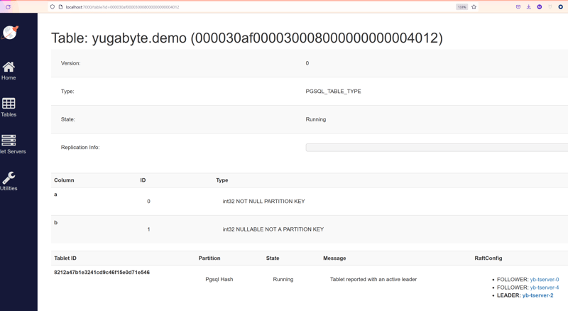
Looking at the console on http://localhost:7000/tables and selecting my demo table I can see the current location of the tablet peers:

I am connected to yb-tserver-0 (docker exec -it yb-tserver-0 ysqlsh) and read from yb-tserver-2 (LEADER: yb-tserver-2). Cross-node calls are expected in a distributed database, to get scalable consistent reads and writes, but we can do better for a reference table which is read mostly.

Duplicate indexes

My goal is to create an equivalent structure (LSM tree on the primary key with all attributes) that is automatically maintained. This will be defined with create unique index on demo(a) include(b). And one in each cloud/node/zone in order to limit the latency for cross-node calls, using the tablespaces I've defined. I'm lazy and generate those statements from my existing tablespaces:

select format('create unique index ind_%s on demo(a) include(b) tablespace %s split into 1 tablets;',spcname,spcname) ddl
from pg_tablespace where spcoptions is not null;

Here is the DDL to create those indexes:

                                                               ddl
----------------------------------------------------------------------------------------------------------------------------------
 create unique index ind_geo_cloud1_region1_zone1 on demo(a) include(b) tablespace geo_cloud1_region1_zone1 split into 1 tablets;
 create unique index ind_geo_cloud1_region1_zone2 on demo(a) include(b) tablespace geo_cloud1_region1_zone2 split into 1 tablets;
 create unique index ind_geo_cloud1_region2_zone1 on demo(a) include(b) tablespace geo_cloud1_region2_zone1 split into 1 tablets;
 create unique index ind_geo_cloud1_region2_zone2 on demo(a) include(b) tablespace geo_cloud1_region2_zone2 split into 1 tablets;
 create unique index ind_geo_cloud2_region1_zone1 on demo(a) include(b) tablespace geo_cloud2_region1_zone1 split into 1 tablets;
 create unique index ind_geo_cloud2_region1_zone2 on demo(a) include(b) tablespace geo_cloud2_region1_zone2 split into 1 tablets;
 create unique index ind_geo_cloud2_region2_zone1 on demo(a) include(b) tablespace geo_cloud2_region2_zone1 split into 1 tablets;
 create unique index ind_geo_cloud2_region2_zone2 on demo(a) include(b) tablespace geo_cloud2_region2_zone2 split into 1 tablets;
(8 rows)

yugabyte=#

The creation may take a few seconds, which may seem long on empty table. There's a reason for that, which I explained in a previous post. Note that I defined only one tablet here (split into 1 tablets) because this is a small table, but all this is using features with many possibilities. It is not excluded that you want to have an index in each zone but distributed to all nodes. And, from the tablespace definition ("num_replicas" : 1) I didn't replicate for High Availability here. In production, you probably want the same replication factor as the table, so that the index is available even when one node is down. The goal of this lab is focused at showing how the query planner chooses the right index. This configuration means that if one node is down, not only the index there is not available, but no update can happen on the table until you drop the index that was on the dead node.

Query using the nearest index

I am still connected to yb-tserver-0 and running the same query as above. Now, rather than reading from demo_pkey (with its leader in yb-tserver-5) it reads from ind_geo_cloud1_region1_zone1:

yugabyte=# explain select * from demo where a=1;

                                          QUERY PLAN
----------------------------------------------------------------------------------------------
 Index Only Scan using ind_geo_cloud1_region1_zone1 on demo  (cost=0.00..4.11 rows=1 width=8)
   Index Cond: (a = 1)
(2 rows)

yugabyte=#

As this is a secondary index, it shows Index Only Scan so that we know that there are no additional hops to read from the table.

The query planner knows where I am connected to, and sees the many possible indexes. it adjusts the cost to favor the nearest zone/region/cloud and picks up the right one. You can see a cost of 4.11 here whereas the read from the primary key was 4.12.

Here is the list of indexes that I have created on my demo table:

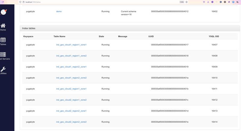
Here is the definition for the one that was picked up:

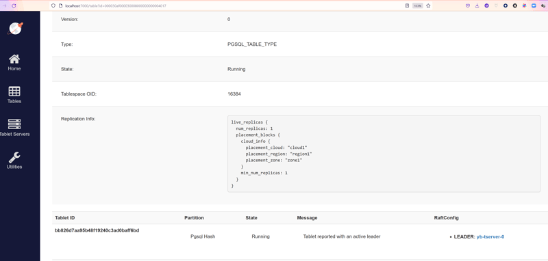
This index has its leader on yb-server-0 which is the same cloud/region/zone I am connected to. And this is visible in "Replication Info" where the placement is inherited from the tablespace.

Explain from all nodes

I've built this lab to easily test this feature on my laptop. This will connect to each node (ysqlsh is the YugabyteDB psql) to show the tserver placement info (from its command line arguments \! ps -p 1 -o cmd), the node it is connected to (\! hostname), and the the execution plan (explain):

for i in {0..7} ; do docker exec -it yb-tserver-$i ysqlsh -c "\\! ps -p 1 -o cmd" -c "\\! hostname"  -c "explain select * from demo where a=1;" ; done

The result shows that each time the nearest index is used.

$ for i in {0..7} ; do docker exec -it yb-tserver-$i ysqlsh -c "\\! ps -p 1 -o cmd" -c "\\! hostname"  -c "explain select * from demo where a=1;" ; done
CMD
/home/yugabyte/bin/yb-tserver --placement_cloud=cloud1 --placement_region=region1 --placement_zone=zone1 --enable_ysql=true --fs_data_dirs=/home/yugabyte/data --tserver_master_addrs=yb-master-0:7100,yb-master-1:7100,yb-master-2:
yb-tserver-0
                                          QUERY PLAN
----------------------------------------------------------------------------------------------
 Index Only Scan using ind_geo_cloud1_region1_zone1 on demo  (cost=0.00..4.11 rows=1 width=8)
   Index Cond: (a = 1)
(2 rows)

CMD
/home/yugabyte/bin/yb-tserver --placement_cloud=cloud2 --placement_region=region1 --placement_zone=zone1 --enable_ysql=true --fs_data_dirs=/home/yugabyte/data --tserver_master_addrs=yb-master-0:7100,yb-master-1:7100,yb-master-2:
yb-tserver-1
                                          QUERY PLAN
----------------------------------------------------------------------------------------------
 Index Only Scan using ind_geo_cloud2_region1_zone1 on demo  (cost=0.00..4.11 rows=1 width=8)
   Index Cond: (a = 1)
(2 rows)

CMD
/home/yugabyte/bin/yb-tserver --placement_cloud=cloud1 --placement_region=region2 --placement_zone=zone1 --enable_ysql=true --fs_data_dirs=/home/yugabyte/data --tserver_master_addrs=yb-master-0:7100,yb-master-1:7100,yb-master-2:
yb-tserver-2
                                          QUERY PLAN
----------------------------------------------------------------------------------------------
 Index Only Scan using ind_geo_cloud1_region2_zone1 on demo  (cost=0.00..4.11 rows=1 width=8)
   Index Cond: (a = 1)
(2 rows)

CMD
/home/yugabyte/bin/yb-tserver --placement_cloud=cloud2 --placement_region=region2 --placement_zone=zone1 --enable_ysql=true --fs_data_dirs=/home/yugabyte/data --tserver_master_addrs=yb-master-0:7100,yb-master-1:7100,yb-master-2:
yb-tserver-3
                                          QUERY PLAN
----------------------------------------------------------------------------------------------
 Index Only Scan using ind_geo_cloud2_region2_zone1 on demo  (cost=0.00..4.11 rows=1 width=8)
   Index Cond: (a = 1)
(2 rows)

CMD
/home/yugabyte/bin/yb-tserver --placement_cloud=cloud1 --placement_region=region1 --placement_zone=zone2 --enable_ysql=true --fs_data_dirs=/home/yugabyte/data --tserver_master_addrs=yb-master-0:7100,yb-master-1:7100,yb-master-2:
yb-tserver-4
                                          QUERY PLAN
----------------------------------------------------------------------------------------------
 Index Only Scan using ind_geo_cloud1_region1_zone2 on demo  (cost=0.00..4.11 rows=1 width=8)
   Index Cond: (a = 1)
(2 rows)

CMD
/home/yugabyte/bin/yb-tserver --placement_cloud=cloud2 --placement_region=region1 --placement_zone=zone2 --enable_ysql=true --fs_data_dirs=/home/yugabyte/data --tserver_master_addrs=yb-master-0:7100,yb-master-1:7100,yb-master-2:
yb-tserver-5
                                          QUERY PLAN
----------------------------------------------------------------------------------------------
 Index Only Scan using ind_geo_cloud2_region1_zone2 on demo  (cost=0.00..4.11 rows=1 width=8)
   Index Cond: (a = 1)
(2 rows)

CMD
/home/yugabyte/bin/yb-tserver --placement_cloud=cloud1 --placement_region=region2 --placement_zone=zone2 --enable_ysql=true --fs_data_dirs=/home/yugabyte/data --tserver_master_addrs=yb-master-0:7100,yb-master-1:7100,yb-master-2:
yb-tserver-6
                                          QUERY PLAN
----------------------------------------------------------------------------------------------
 Index Only Scan using ind_geo_cloud1_region2_zone2 on demo  (cost=0.00..4.11 rows=1 width=8)
   Index Cond: (a = 1)
(2 rows)

CMD
/home/yugabyte/bin/yb-tserver --placement_cloud=cloud2 --placement_region=region2 --placement_zone=zone2 --enable_ysql=true --fs_data_dirs=/home/yugabyte/data --tserver_master_addrs=yb-master-0:7100,yb-master-1:7100,yb-master-2:
yb-tserver-7
                                          QUERY PLAN
----------------------------------------------------------------------------------------------
 Index Only Scan using ind_geo_cloud2_region2_zone2 on demo  (cost=0.00..4.11 rows=1 width=8)
   Index Cond: (a = 1)
(2 rows)

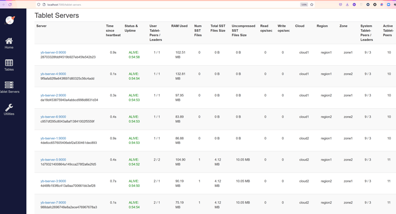
You can easily see the map of servers / placement from yb_servers() or the console http://localhost:7000/tablet-servers:

Cost-based decision explained with hints

When connected to yb-server-0 I'll force each index with a hint to show the associated cost. I've run analyze demo and I generate the queries with:

yugabyte=#
select format('explain /*+ IndexOnlyScan(demo %I) */ select * from demo;',indexname) from pg_indexes where tablename='demo' and indexname != 'demo_pkey';

Here are the queries and the result:

yugabyte=#  explain /*+ IndexOnlyScan(demo ind_geo_cloud1_region1_zone1) */ select * from demo;
                                              QUERY PLAN
-------------------------------------------------------------------------------------------------------
 Index Only Scan using ind_geo_cloud1_region1_zone1 on demo  (cost=0.00..10404.00 rows=100000 width=8)
(1 row)

yugabyte=#  explain /*+ IndexOnlyScan(demo ind_geo_cloud1_region1_zone2) */ select * from demo;
                                              QUERY PLAN
-------------------------------------------------------------------------------------------------------
 Index Only Scan using ind_geo_cloud1_region1_zone2 on demo  (cost=0.00..10504.00 rows=100000 width=8)
(1 row)

yugabyte=#  explain /*+ IndexOnlyScan(demo ind_geo_cloud1_region2_zone1) */ select * from demo;
                                              QUERY PLAN
-------------------------------------------------------------------------------------------------------
 Index Only Scan using ind_geo_cloud1_region2_zone1 on demo  (cost=0.00..11004.00 rows=100000 width=8)
(1 row)

yugabyte=#  explain /*+ IndexOnlyScan(demo ind_geo_cloud1_region2_zone2) */ select * from demo;
                                              QUERY PLAN
-------------------------------------------------------------------------------------------------------
 Index Only Scan using ind_geo_cloud1_region2_zone2 on demo  (cost=0.00..11004.00 rows=100000 width=8)
(1 row)

yugabyte=#  explain /*+ IndexOnlyScan(demo ind_geo_cloud2_region1_zone1) */ select * from demo;
                                              QUERY PLAN
-------------------------------------------------------------------------------------------------------
 Index Only Scan using ind_geo_cloud2_region1_zone1 on demo  (cost=0.00..11004.00 rows=100000 width=8)
(1 row)

yugabyte=#  explain /*+ IndexOnlyScan(demo ind_geo_cloud2_region1_zone2) */ select * from demo;
                                              QUERY PLAN
-------------------------------------------------------------------------------------------------------
 Index Only Scan using ind_geo_cloud2_region1_zone2 on demo  (cost=0.00..11004.00 rows=100000 width=8)
(1 row)

yugabyte=#  explain /*+ IndexOnlyScan(demo ind_geo_cloud2_region2_zone1) */ select * from demo;
                                              QUERY PLAN
-------------------------------------------------------------------------------------------------------
 Index Only Scan using ind_geo_cloud2_region2_zone1 on demo  (cost=0.00..11004.00 rows=100000 width=8)
(1 row)

yugabyte=#  explain /*+ IndexOnlyScan(demo ind_geo_cloud2_region2_zone2) */ select * from demo;
                                              QUERY PLAN
-------------------------------------------------------------------------------------------------------
 Index Only Scan using ind_geo_cloud2_region2_zone2 on demo  (cost=0.00..11004.00 rows=100000 width=8)
(1 row)

From yb-server-t0 which is in cloud1.region1.zone1 the estimated cost to read all 100000 rows via IndexOnlyScan is:

cost=0.00..10404.00 from ind_geo_cloud1_region1_zone1 which is in the local zone
cost=0.00..10504.00 from ind_geo_cloud1_region1_zone2 which is in a different zone but the same region
cost=0.00..11004.00 from other indexes when are in different cloud regions.

This is the simple way the optimizer favors local indexes when having the choice.

Updates on the reference table

Please, remember that this solution is for infrequent writes, on small reference tables. Here, with 8 copies in all zones (which is extreme), an update demo set b=2; shows how all servers are busy:

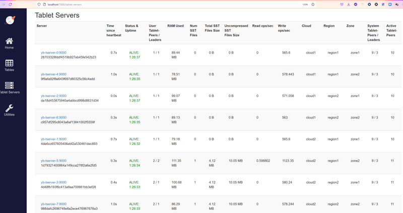
Nearly 600 write operations per second to the index leaders in each node, and the double on yb-tserver-5 which also holds the table leader.

You must balance the cost of updates with the performance of writes. For a small table that is read often and rarely updated, one index per zone is a possibility. For larger tables with large updates, maybe one per region is a better tradeoff.

Current limitations

This post shows how to test and reproduce as you will probably try this on a newer version and YugabyteDB eveloves very fast. This is on version 2.11. If you see some limitations, please comment here or open a git issue: https://github.com/yugabyte/yugabyte-db

Colocated tables

I mentionned that you cannot use this on colocated table because indexes are also colocated. If you do, you will see the same result as above (the right index being used) but it will not avoid cross-node calls because all duplicated indexes will be at the same place.

Seq Scan

The duplicate index Index Only Scan is favored over the primary key Index Scan but not over a Seq Scan even if the actual cost could be lower when coming from a local node:

yugabyte=# explain select * from demo;

                       QUERY PLAN
---------------------------------------------------------
 Seq Scan on demo  (cost=0.00..100.00 rows=1000 width=8)

yugabyte=# explain /*+ IndexOnlyScan(demo ind_geo_cloud1_region1_zone1) */ select * from demo;

                                            QUERY PLAN
---------------------------------------------------------------------------------------------------
 Index Only Scan using ind_geo_cloud1_region1_zone1 on demo  (cost=0.00..108.00 rows=1000 width=8)
(1 row)

Thanks to hints, we can show that the Index Only Scan from the duplicate index is a possible access path, but estimated with a higher cost.

UNIQUE index

You may wonder if you need a unique index, so let's try with a non-unique one:

yugabyte=# \d demo
                Table "public.demo"
 Column |  Type   | Collation | Nullable | Default
--------+---------+-----------+----------+---------
 a      | integer |           | not null |
 b      | integer |           |          |
Indexes:
    "demo_pkey" PRIMARY KEY, lsm (a HASH)
    "ind_geo_cloud1_region1_zone1" UNIQUE, lsm (a HASH) INCLUDE (b), tablespace "geo_cloud1_region1_zone1"
    "ind_geo_cloud1_region1_zone2" lsm (a HASH) INCLUDE (b), tablespace "geo_cloud1_region1_zone2"
    "ind_geo_cloud1_region2_zone1" lsm (a HASH) INCLUDE (b), tablespace "geo_cloud1_region2_zone1"
    "ind_geo_cloud1_region2_zone2" lsm (a HASH) INCLUDE (b), tablespace "geo_cloud1_region2_zone2"
    "ind_geo_cloud2_region1_zone1" lsm (a HASH) INCLUDE (b), tablespace "geo_cloud2_region1_zone1"
    "ind_geo_cloud2_region1_zone2" lsm (a HASH) INCLUDE (b), tablespace "geo_cloud2_region1_zone2"
    "ind_geo_cloud2_region2_zone1" lsm (a HASH) INCLUDE (b), tablespace "geo_cloud2_region2_zone1"
    "ind_geo_cloud2_region2_zone2" lsm (a HASH) INCLUDE (b), tablespace "geo_cloud2_region2_zone2"

yugabyte=# explain select * from demo where a=1;

                                          QUERY PLAN
----------------------------------------------------------------------------------------------
 Index Only Scan using ind_geo_cloud1_region1_zone1 on demo  (cost=0.00..4.11 rows=1 width=8)
   Index Cond: (a = 1)
(2 rows)

yugabyte=# drop index ind_geo_cloud1_region1_zone1;
DROP INDEX

yugabyte=# explain select * from demo where a=1;

                              QUERY PLAN
----------------------------------------------------------------------
 Index Scan using demo_pkey on demo  (cost=0.00..4.11 rows=1 width=8)
   Index Cond: (a = 1)
(2 rows)

yugabyte=#  create       index ind_geo_cloud1_region1_zone1 on demo(a) include(b) tablespace geo_cloud1_region1_zone1 split into 1 tablets;
CREATE INDEX
yugabyte=# explain select * from demo where a=1;

                              QUERY PLAN
----------------------------------------------------------------------
 Index Scan using demo_pkey on demo  (cost=0.00..4.11 rows=1 width=8)
   Index Cond: (a = 1)
(2 rows)

yugabyte=# explain /*+ IndexOnlyScan(demo ind_geo_cloud1_region1_zone1) */ select * from demo where a=1;


                                          QUERY PLAN
-----------------------------------------------------------------------------------------------
 Index Only Scan using ind_geo_cloud1_region1_zone1 on demo  (cost=0.00..5.06 rows=10 width=8)
   Index Cond: (a = 1)
(2 rows)

So, yes UNIQUE index is mandatory if you want the query planner to choose your duplicate index, because the cost from a non-unique index is estimated higher than from the primary key. But it can be used with hint.

INCLUDE index

Index Only Scan doesn't need an INCLUDE index. The additional columns can be in the key and it will still be unique. INCLUDE is mostly there to enforce a unique constraint on a subset of the columns, but in this case, the table already enforces it with the primary key.

yugabyte=# drop index ind_geo_cloud1_region1_zone1;
DROP INDEX

yugabyte=#  create unique index ind_geo_cloud1_region1_zone1 on demo(a,b) tablespace geo_cloud1_region1_zone1 split into 1 tablets;
CREATE INDEX

yugabyte=# explain select * from demo where a=1;

                              QUERY PLAN
----------------------------------------------------------------------
 Index Scan using demo_pkey on demo  (cost=0.00..4.11 rows=1 width=8)
   Index Cond: (a = 1)
(2 rows)

yugabyte=# explain /*+ IndexOnlyScan(demo ind_geo_cloud1_region1_zone1) */ select * from demo where a=1;

                                           QUERY PLAN
-------------------------------------------------------------------------------------------------
 Index Only Scan using ind_geo_cloud1_region1_zone1 on demo  (cost=0.00..14.65 rows=100 width=8)
   Index Cond: (a = 1)
(2 rows)

Here, again, the duplicate index can be used with a hint but is not chosen by the query plannder because the cost of an index with a larger key is higher.

Again, if you think those limitations are a problem, open a git issue to explain your use case.

In summary

As a distributed SQL database, YugabyteDB will, by default, distribute data across all nodes. But you have many controls on the placement, using the SQL features: tables, indexes, tablespaces. The cost-based query planner will take the best decision at runtime, but you can also control it with hints. This gives much more agility than a simple distributed table /reference table flag, because OLTP application are complex. This technique can be used in any cloud or on-premises configuration, on primary or secondary indexes, is declarative within the database, with node need to change the code.

Reference Tables as duplicate covering indexes